What does multiDA actually do?

The multiDA model

We illustrate the main workings of the multiDA model in simplicity for this vignette. Please see the pre-print here for a more detailed exposition.

Describing the data

Suppose you have data \(\textbf{X}\) of dimension $ n p$, with a corresponding response vector \(\textbf{y}\) of length \(n\) describing class membership for each observation.

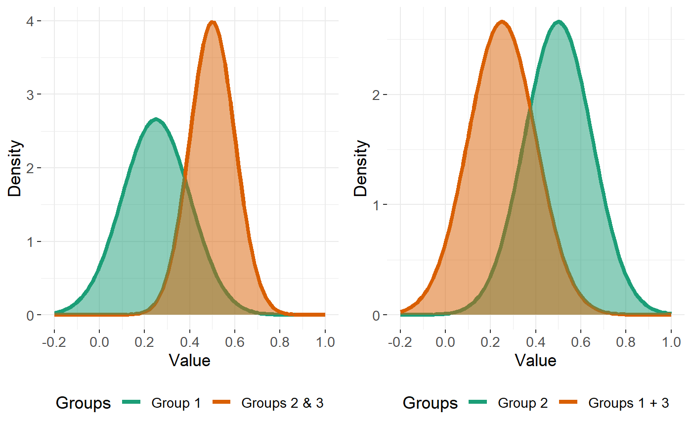
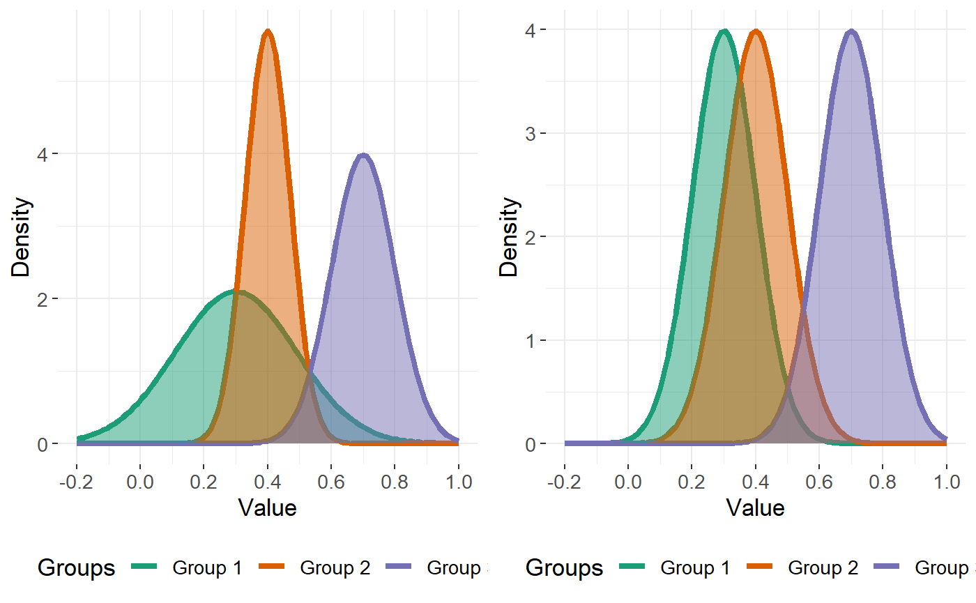
Further suppose, for this example, our response consists of \(K=3\) classes, and we wish to describe each feature \(j\) by a combination of \(1, 2,\) or \(3\) Gaussian distributions for each class. How can we do this? Let’s consider the cases that can occur for each feature \(j\).

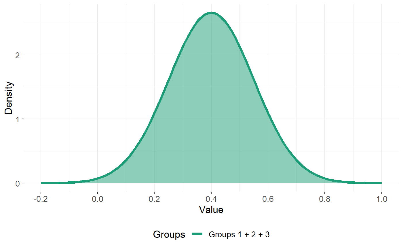
Case 1 - all of the classes can be described by a single Gaussian curve

This corresponds to the case of the feature being non-informative.

Case 2 - two of the classes can be combined into a Gaussian curve, the other is left behind (one vs rest)

This corresponds to an informative/significant feature. We can either allow each curve to have different variances (left), or restrict the curves to have equal variances (right).

Case 3 - each of the three classes are distinct.

This corresponds to an informative/significant feature. Again, we can either allow each curve to have different variances (left), or restrict the curves to have equal variances (right).

A Penalised Likelihood Ratio Test to determine appropriate group structure for each feature

The multiDA model uses a penalised likelihood ratio test to determine which group structure as described above best describes each feature. The penalisation process is described in detail in the paper. The two penalty options available for this algorithm are the BIC (Schwarz, 1978), and the Extended BIC (EBIC - Chen and Chen, 2008). The EBIC penalty is the default, and is a stronger (and more appropriate) penalty for high dimensional data.

Prediction

Assuming a multinomial distribution for the response vector \(\textbf{y}\), the multiDA algorithm uses information from a trained model (described above) to predict the probability of class membership for each class for a new datapoint. A probability matrix can be returned, or the value of the most probable class.